Chapter 6. Competition

Intraspecific competition -within [W/I] population:

The logistic growth curve for intraspecific competition (see Chapter 5),
dN/dt = rN_(t-1)*(K - N_t)/K
has been confirmed, by Park (1948) and Nicholson (1954), to describe accurately the population growth and eventual achievement of a stable population density in laboratory situations with a single species presented with a limited food supply. It should be noted that the laboratory experiments were highly simplified compared to the natural world: it was bounded by walls, had very little environmental variation (such as no diurnal temperature cycle), no opportunity for either emigration nor immigration, no predators, …. Because it was a model of intraspecific competition in isolation, the results may not have much bearing on the nature of intraspecific competition in the ecosystem. However, it did contribute greatly to the development of a theoretical understanding of competition, and served to support Darwin's assertion that a struggle for existence occurs and is probably the most intense within the populations of a single species.

Interspecific competition -between [B/T] populations:

This mathematical model was later expanded to include 2 (or more species) as
dN₁/dt = rN_1,(t-1)*(K₁ - N_1,t - b_2,1*N_2,t)/K₁
dN₂/dt = rN_2,(t-1)*(K₂ - N_2,t - b_1,2*N_1,t)/K₂,
where b_2,1 and b_1,2 are, respectively, correction factors showing the equivalent population of species 2 in terms of species 1 and the equivalent population of species 1 in terms of species 2, recognizing the difference in demands on the environment by each species. This is similar to the BLM (U. S. Bureau of Land Management) range management livestock equivalent ‘standard grazing unit’ (1 cow and 1 calf = 2 sheep and 1 lamb), so b_sheep,cow = 0.6 cows and b_cow,sheep = 1.7 sheep.
    Park (1948) designed a series of laboratory experiments in which two distinct species were presented with a limited food resource to test these modified logistic growth curves. When each species was grown separately, the origninal logistic growth curve accurately predicted the growth of the confined populations to a stable equilibrium. Then, when the two species were grown together, the modified logistic growth curves matched the observed growth of the each population. At a seminar I attended, it was suggested that the logistic growth curve could be ‘generalized’ as
dN₁/dt = rN_1,(t-1)*(∑(K_i) - N_1,t - ∑(b_i,1*N_i,t)/∑(K_i)
where ∑(K_i) is the sum of K for all competing species which suggests the third definition (in the glossary) of carrying capacity (the capacity of the enviroment to support the populations of all species, stated in terms of the sum of the populations of all species present).

Hypotheses based on experiments and field studies

The proposed theoretical mechanisms driving competition as just described suggested that there need to be three possible models to account for competition in natural populations.
    Model 1. “All competitors get a small amount of resource.”
The amount of the limited resource(s) received by the individuals is insufficient for all members of the population, resulting in reduced reproduction across the entire population.
    Model 2. “A fraction of competitors get all resources needed.”
This also means that the other fraction of the competitors receive an insufficient amount of the resources to support survival. The potential effects on those not getting full resources include reduced growth, fecundity (reproduction), or survival (self-thinning). Applying Darwin's “survival of the fittest” principle, if the fraction receiving all of the resources needed are associated with an inheritable trait, then we would expect an evolutionary event to occur. Even if those individuals not receiving adequate resources have behavioral rather than physiological responses, such as increased dispersal (avoidance), altered social dominance structure (peck order), or greater territoriality (defense of a subsite from competitors) & increased home range (subsite where the search for food resources occurs); the population of individuals receiving adequate resources can still undergo evolutiionary alterations.
    Model 3. “Density Independent mechanisms determine how many individuals compete for the resources.”
These generally involve cyclic (or periodic) changes the resources available, such as the short-term climate cycling between conditions favorable to the population and conditions unfavorable to it; predator migrations (changing the death rate); and fluctuations in available foos species biomass (which also changes the death rate of the population under consideration).

Niche

The Competitive Exclusion Principle

The logistic growth curves for two species which have identical demands on the environment, but have different reproductive potential (r₁ & r₂ in the equations), predicts that the population of the species with the higher r-value will eventually reach K_i, while the population of the species with the lower r-value will drop to zero (these two values, K & zero, are the only stable solutions to the equations). This was described [“Gause's contention (1934) that two species with similar ecology cannot live together in the same place,” G. Hardin 1960. “The Competitive Exclusion Principle,” Science vol 131, no 3409 (29 April 1960) pp. 1292-1297] as the competitive exclusion principle. Since communities (the populations of all species [usually of a single high level taxon, such as Order] occupying the same site) actually exist, competitive exclusion either does not happen or is not correctly stated. To resolve the apparent contradiction, Ecologists developed the concept of the niche defined as the specific details of the habitat which support one species, but not the other species of the same community, and re-worded the competitive exclusion principle as “two species with the same niche cannot live together in the same place.” We may have now reduced the competitive exclusion principle (and niche) to a tautology. [“A tautology is a logical statement in which the conclusion is equivalent to the premise.” downloaded on 10 Feb 2011 from mathworld.wolfram.com/Tautology.html].
    There are, however, some field data which strongly suggest that the principle does describe the behavior of species in natural systems. One example which clearly illustrates this is the Tufted titmouse (Parus bicolor) - Black-capped chickadee (Parus atricapillus) interactions (Lack, 1971). Both birds occupy similar woodlands (often coexisitng in the same woods), eating similar insects; but one species tends to nest and feed among the smaller branches and twigs near the edge of the tree canopy, while the other tends to nest and feed among the larger branches near the trunk of the tree. This could be taken as a demonstration of the competitive exclusion principle. The best known example of the principle is exotic (or invasive) species displacing the native species from their niches. In most cases the invasive species has driven the native species to the brink of local extinction, but there are several cases in which the native species appears to have been driven to global extinction. In addition, there are cases where the field data suggest that the principle does not apply, with two competing species persisting in the same site at rather high population densities for extended time periods. These cases have generally been explained as a variable environment, such as cyclic wet/dry climates, alternately favoring one or the other of the two species. In this scenario, neither species has time to decline much under the unfavorable conditions before the environment shifts back to favor that species.

Niche:

Niche width is used to describe the full range of environmental conditions within which the species can compete successfully and maintain populations densities close to the carrying capacity of the species. It is expected that the species may have lower carrying capacities toward the “edges” of the niche.

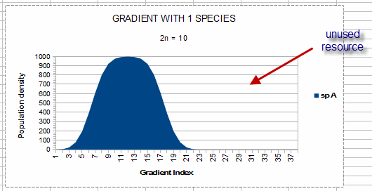
In this illustration, the niche width is from gradient index = 2 to gradient index =22. The “gradient index” will be explained in Chapter 9; for now it simply represents the level of the environmental factor. The unshaded portion of the graph is ‘unused resource,’ which is available for other species without competition.
Niche width is a function of the number of genes which determine fitness. For Plants, this number could be fairly large because Plants can undergo “autopolyploidy,” in which the number of chromosomes doubles spontaneously. This also doubles the number of genes for each trait, because each chromosome and its double initially have the exact same genes and alleles. If we assume that there is a gene for adaptation to the environment on each chromosome, the number of different phenotypes [in this case the gradient index or level of environmental factors] will be 2n + 1 [where n is the number of chromosome pairs]. For the illustrations here, I have modelled the species carrying capacity distribution for a species (sp A) with 5 pairs of chromosomes, with the response (population density) distribution for each phenotype as a Normal distribution (with the means slightly displaced and with the same variance). The species response curve is the sum of the response curves for each of the 2n+1 = 11 phenotypes.
    When we take the carrying capacity as the ability of the environment to support all species, it is possible that the species will take a large portion of the environmental resources in its optimum range, but toward the edges of the niche may take a smaller portion of the carrying capacity for all species.

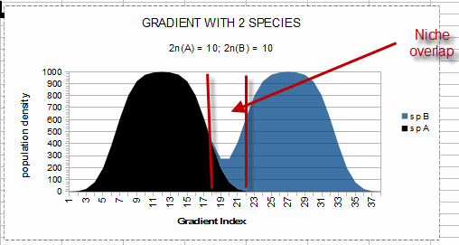
The distribution of a second species (sp B) is shown as being added to the distribution (above the graph for sp A).
In this interpretation, the edge of another species (sp B) niche may overlap the edge of the first species (sp A) niche (the area between the vertical red lines in the graph, or gradient index = 18 to 22) allowing both species to persist indefinitely in the area of “niche overlap,” since both species reach their respective carrying capacity without the combined demands of the two species reaching the ability of the environment to support all species (the top of the graph, or population density = 1000). Notice that there is ‘unused resource’ between sp A and sp B, so an additional species could be squeezed between them as long as the combined maximum expected populations of all three species is less than the capacity of the environment to support all species. However, when the combined populations of all species at any gradient index value exceeds the total capacity of the environment to support all species at that gradient index value, competition will take place but may result in populations less than what could occur in the absence of competition without the less fit species declining to zero population (as predicted by the calculus-based logistic growth equations). The interpretation I am suggesting here allows for any (or all) species to persist at less than their full potential as long as resources are available to support their reduced population density.

niche dynamics

The niche is not considered to be a static characteristic of a population, but can (and does) change. “Niche compression,” or a reduction in niche width, occurs when the habitat is invaded by an exotic species. As the new species out-competes the former species, the former species will occupy a smaller niche. Conversely, “niche expansion,” or ecological release, occurs when a former competitor has become extinct or when the species immigrates to a new habitat. A “niche shift,” as the name suggests, would require the species to change its niche, usually to avoid competition.

RETURN to
  ECOLOGY Outline
  TwoOldGuys HOME

© 2010 TwoOldGuys ™

revised: 09 Feb 2011